It’s probably complicated: Visualising the states of a quantum computer

This is a devlog for the project QByte, but rather than a straight devlog, I’m taking a topic I’ve encountered and delving into it. At the end, I’ll do a brief run-down of my last couple of weeks.

You can find this week’s build for QByte here.

Normal, classical, digital states are quite simple: a bit can either be 1 or 0, which means that 2 bits can have 4 values (00, 01, 10, 11), 3 bits can have 8 and so on.

A single quantum bit, on the other hand, is represented by 2 somewhat arbitrary numbers. It is 0, or 1, or a combination of both. 2 qubits is represented by 4 numbers (a number for each of the 4 values of 2 classical bits), 3 qubits by 8 numbers, and so on.

To make matters simultaneously better and worse, the mathematical representation that we’re using for states in QByte are density matrices: which are basically 2^n by 2^n grids of numbers (so 2x2 for 1 bit, 4x4 for 2 bits, 8x8 for 3 bits etc.). Density matrices are really good in that they neatly package the data we most care about (the probabilities of different states).

Density Matrices for 1-bit states

What all of this means is that visualising quantum states is, at best, a complicated affair, but it’s also the key to making QByte work.

Feedback and Understanding

If there’s a key conceit behind the QByte project, it’s that with sufficient motivation and feedback, a person playing with a quantum computer simulation can grow to understand the underlying mechanics of quantum computing.

The motivation part is the job of the metaphor and the player goals, but without good feedback, it’s not possible to convert player actions into learning. This is where QByte stands out from most quantum computing tools: in most tools, you have to build the whole circuit, set up the inputs and then run the program to see what happens. In QByte, the player gets immediate feedback about how each change affects the state of each bit, and how that affects all the states down the line.

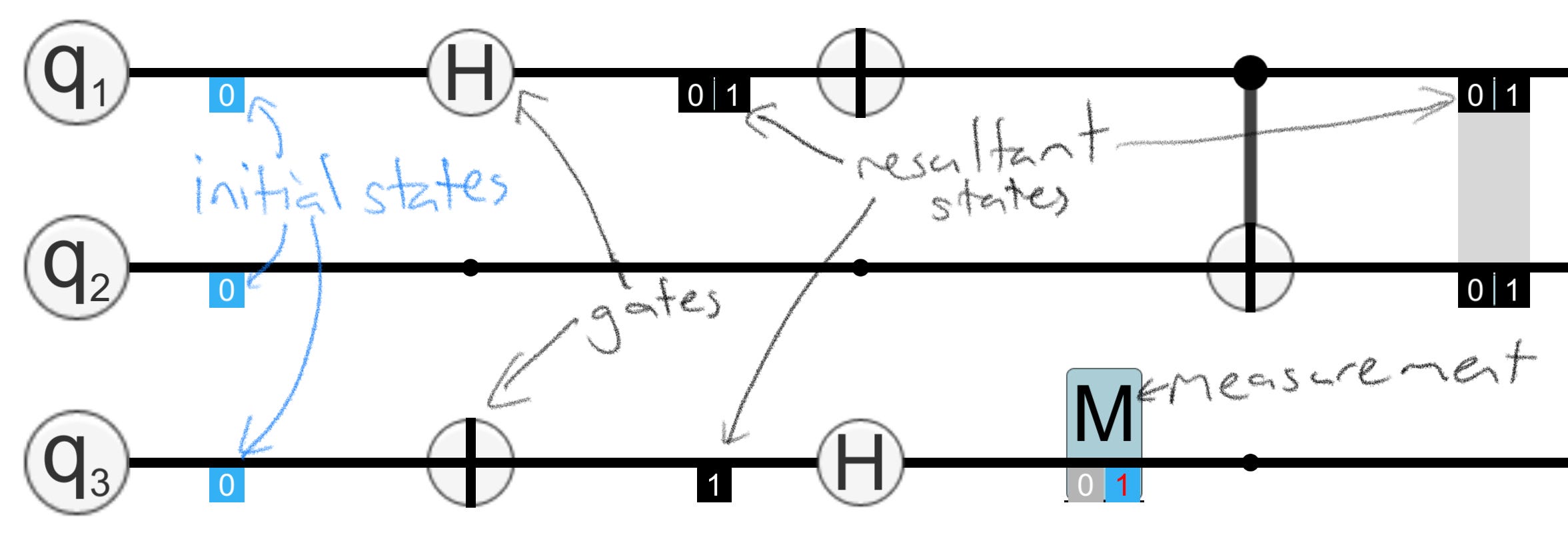In QByte, states are shown whenever they change

To do this, QByte represents the state of each bit at the start of the circuit and whenever it changes. Because circuits should be able to take variable input, input states can be changed by the user – this let’s players try different possible inputs and learn how the circuit will react. At the start, players will mostly be thinking about static inputs, but hopefully, with time, they can begin to play with dynamic inputs as well.

Part 1: Information

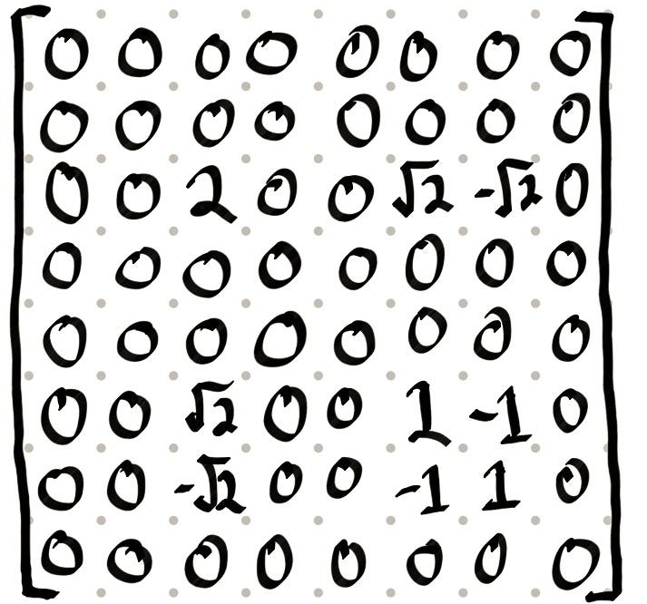A density matrix for a 3-bit state

As mentioned before, density matrices can be pretty large structures — there’s quite a bit of information encoded here.

To represent this visually, I had to cull some data — there’s only so much information a person can parse before it gets too complex, and I want to be able to put these on every state.

Which meant that I needed to develop an information hierarchy, which looks something like this:

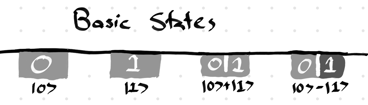
1. Players care most about basic probabilities: how likely is a bit to be 0 or 1

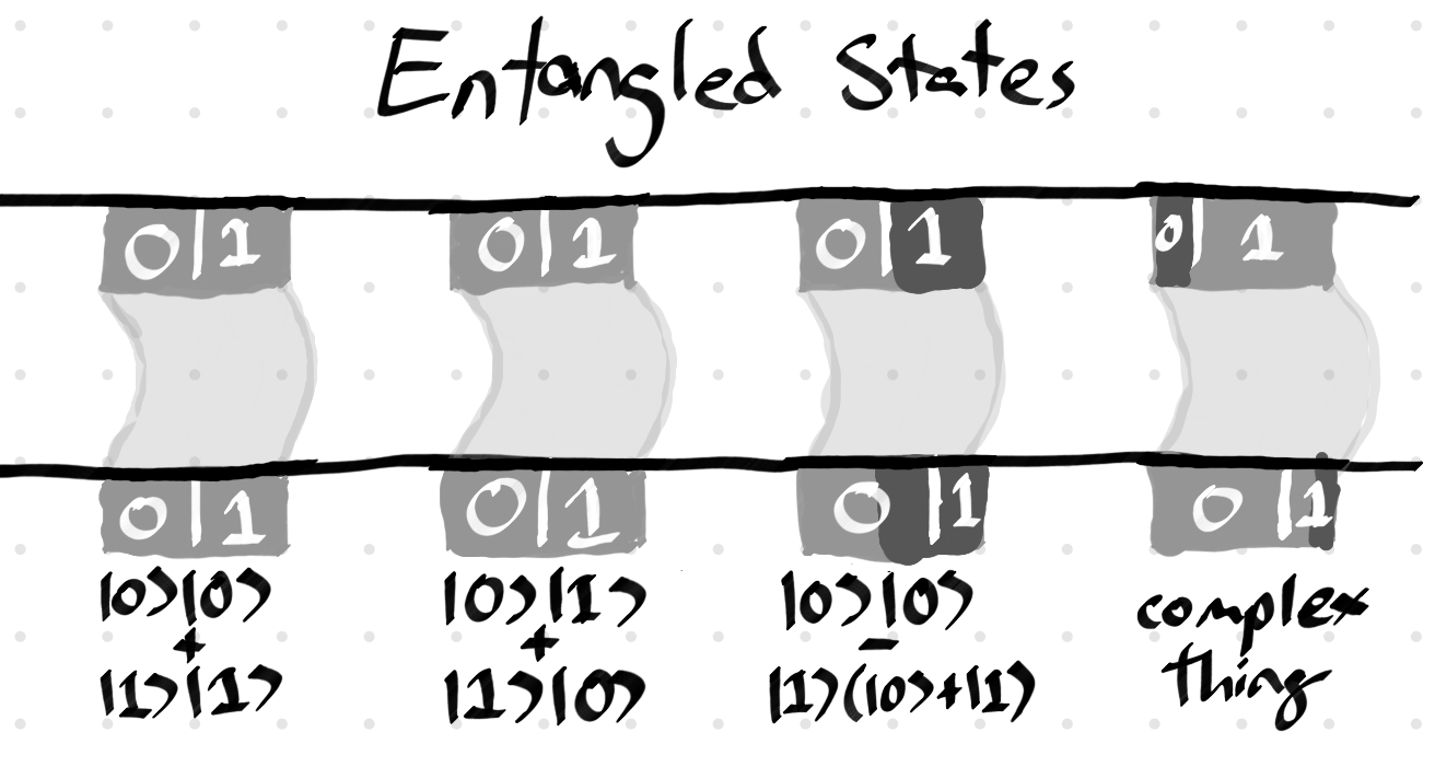
2. They then care about how that choice will affect the values of other bits (ie. entanglements). It’s more important to know which bits are entangled than the details of that entanglement

3. Finally, we need to be able to differentiate between different states that have the same properties for the first two

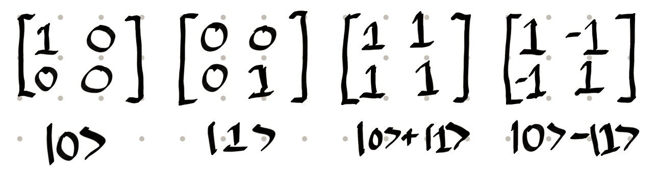
Probabilities

Thankfully, density matrices are great for this: we can simply read the diagonal entries (top left to bottom right) of the matrix to work out the relative probabilities of different states. In the example above, the |0>|1>|0> state (meaning that the first bit is 0, the second is 1, and the third is 0) has probability 2, while |1>|0>|1> and |1>|1>|0> both have probability 1. All other possibilities have a probability of 0.

Note that this is an example of 3 entangled qubits — that means that if one of them is measured, it affects the other two (for instance, if the second bit is measured as |0>, the first and third are definitely |1>). The QByte engine automatically separates states that aren’t entangled, so if we’ve got a density matrix for 3 bits, it means that these bits are entangled.

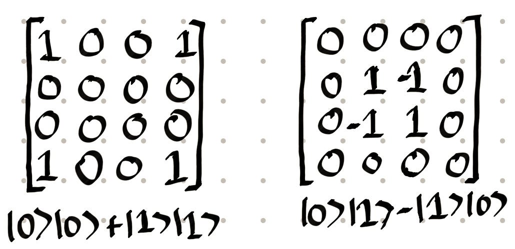Two fairly similar entangled states for 2 bits

Entanglements

How they are entangled is important information that the user needs to know. In both examples above, there is a 50% chance that each bit is |0>, and a 50% chance that it is |1>. However, the bits on the left will always agree with each other, while the bits on the right will always disagree.

Not-Quite-Equivalent States

At this stage, it looks like we can probably throw out the non-diagonal entries for our visualisation, but we can’t quite do it yet.

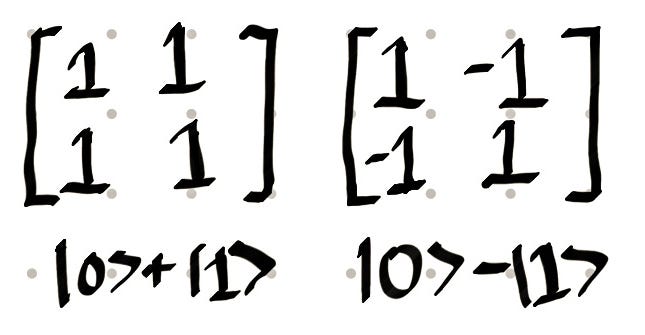The |+> and |-> states

The states to the left have identical diagonal entries: that is, they’ve both got a 50% chance of being |0> or |1>. But their diagonal entries are different, and the (very strange) truth is that these two states are as different from each other than |0> is from |1>. In fact, if you apply a Hadamard gate (a fairly standard gate) to both, the left state turns int |0>, and the right one turns into |1>.

The important thing for us to take are the minus signs: it gives us information about the relationship between the different possibilities. We can use them to assign a sign to each of the diagonal entries using this information, and then throw out the non-diagonal entries. We can also throw out the diagonal entries that are 0.

What we’re left with is what I call ‘State Pieces’, each of which is based on a diagonal entry. Each piece tells us the probability of a specific combination of values, as well as whether that combination is positive or negative.

* The sign associated with a diagonal entry is relative to other entries — there’s no absolute positive or negative here. It also doesn’t affect the base probabilities at all.

** A big reason why we’re able to throw out this information is an earlier decision in the project: that we’re not going to use complex numbers. This saves us a whole lot of headaches, including this one.

Part 2: Visualisation

All of the pieces

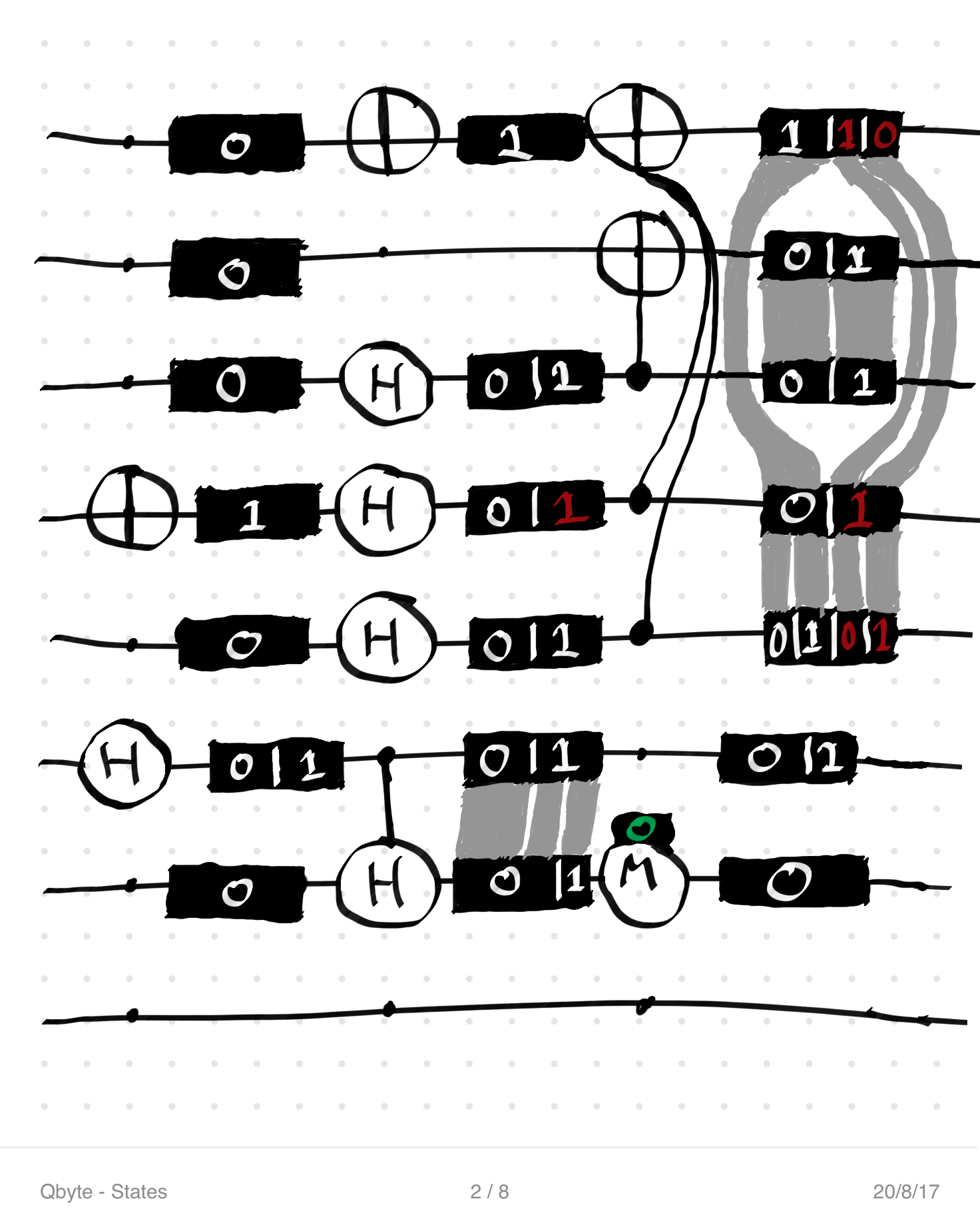
The first implementation of state representations was quite simple: represent each State Piece as a bar on each bit, and use the probabilities to determine the length of the bar. Turn the text on negative pieces red.

The first approach for QByte’s state representations

This approach has a few advantages:

• the states can be small when they aren’t complicated (for instance, the initial states)

• the spaces between gates is constant

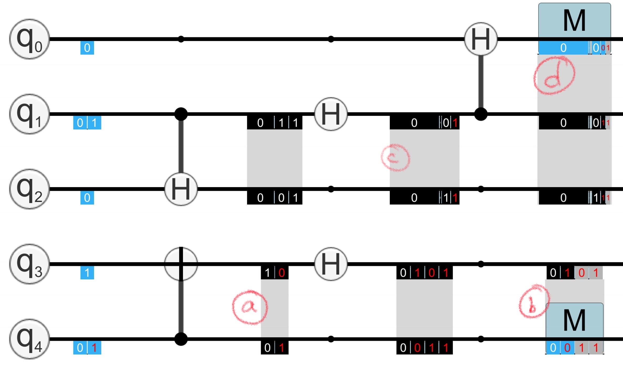
• entangled pieces line up, making it quite easy to tell how one bit’s state affects another (in state (a), it’s clear that q3 and q4 disagree)

• measurements can simply highlight the measured parts of the state, without having to represent the new state separately (in state (b), the greyed out pieces are those which weren’t measured)

However, there’s also a few problems:

• When there’s lots of pieces or those pieces have low probabilities, they become impossible to read (see states (c) and (d))

• The bars that connect bits to show entanglement can get confusing

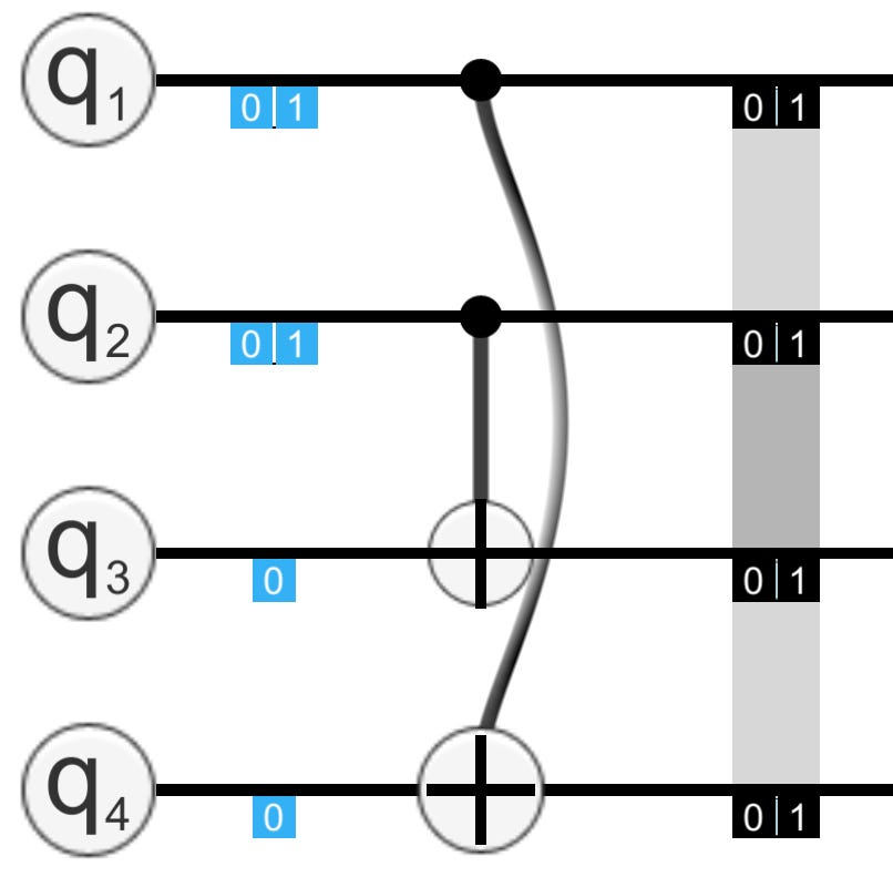It’s hard to tell from the state alone whether q1 is entangled with q3 or q4.

• The representation breaks our information hierarchy — once the states get a little bit complicated, it gets quite hard to read the probability of a bit being |0> or |1> from the diagram (which is, as you recall, the most important piece of information).

Concepts Galore

At this stage, I took a bit of time to try out some concepts on paper. These were all based on a single circuit, which I’d designed to have a decent mix of different types of states.

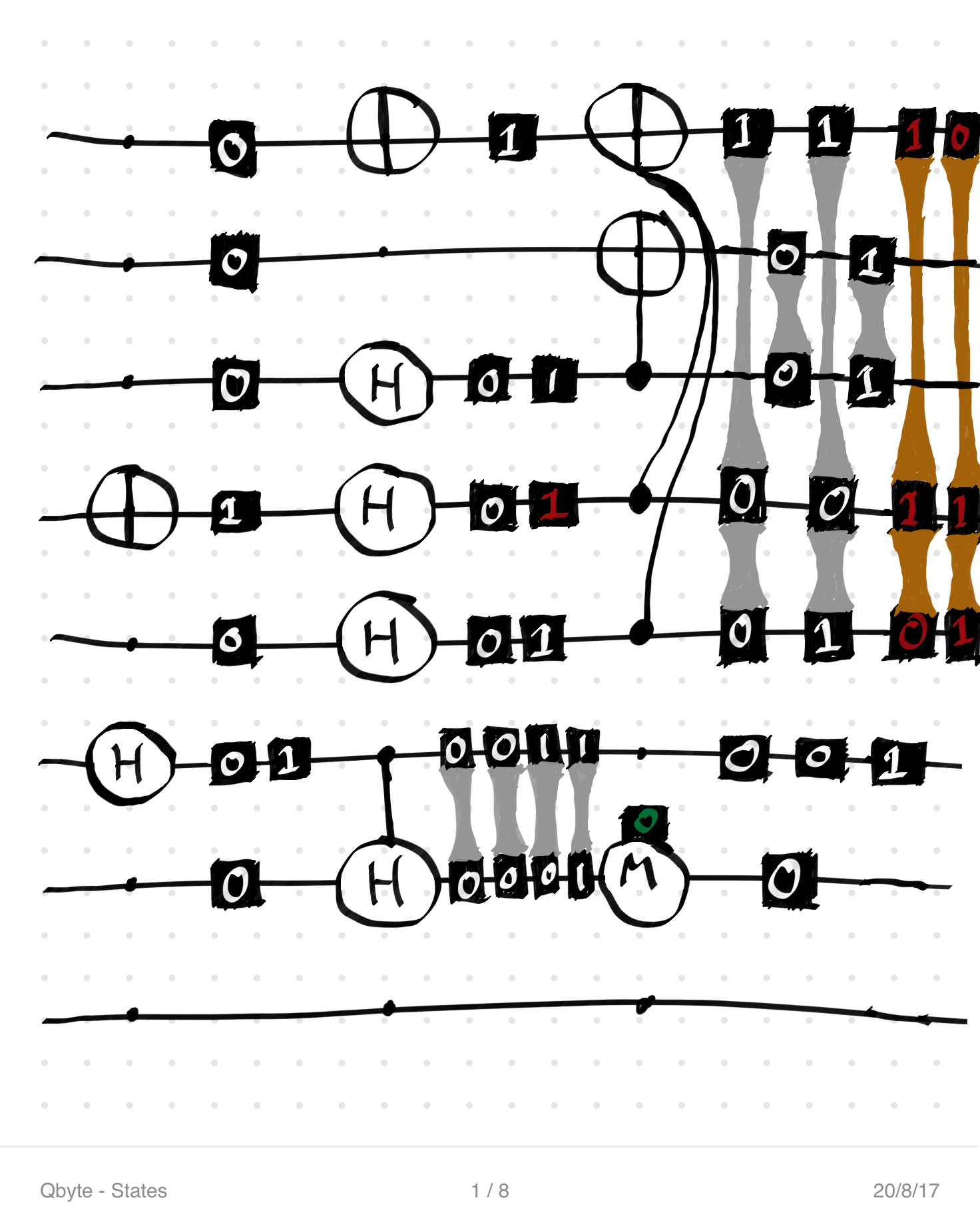
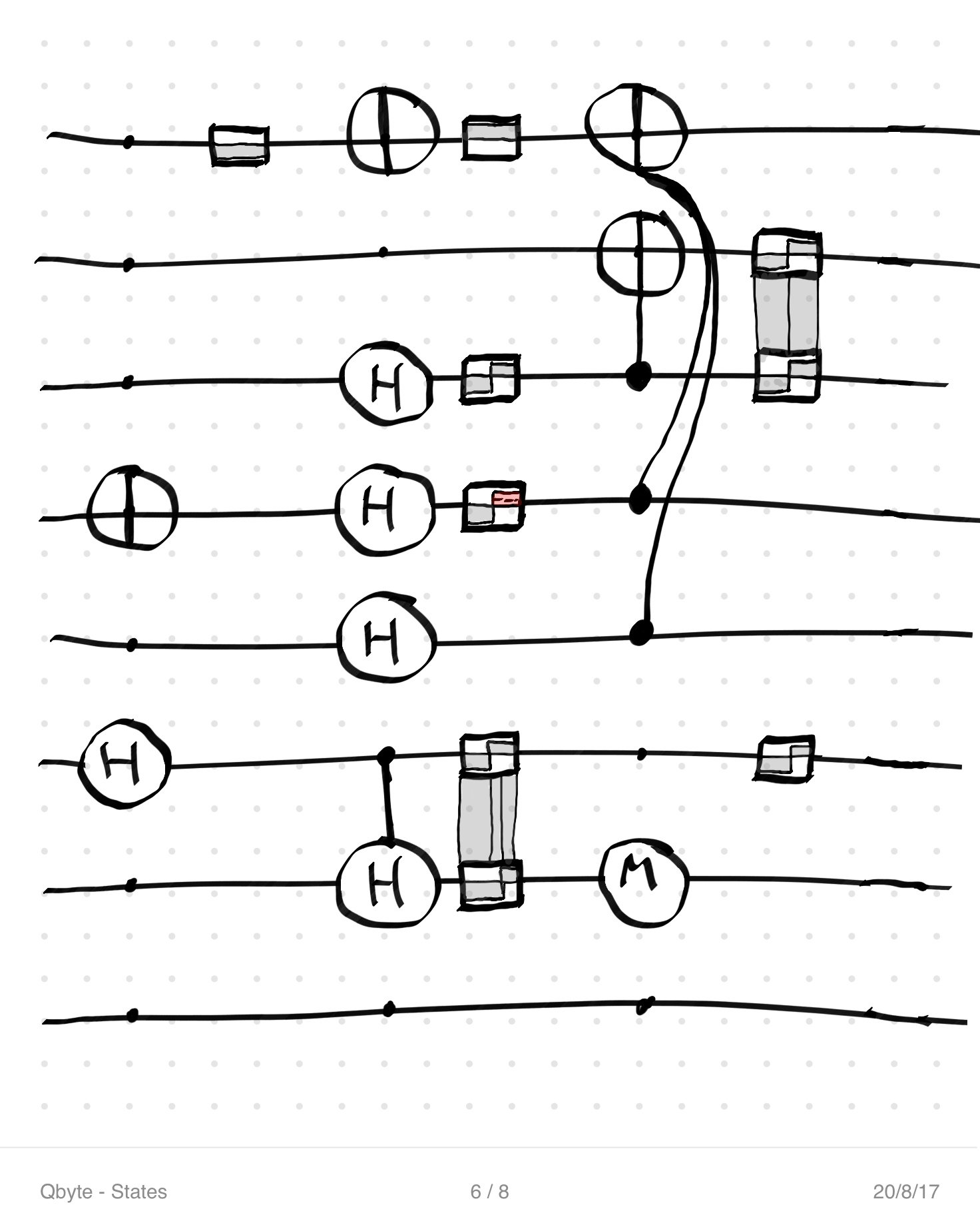Some different concepts for state representations

The issue with most of these was that they became too difficult to read once entanglements became more complicated (I didn’t even bother drawing some of the states for the representation on the right, because I had no idea how I’d do it). Trying to fit all of the information on the representation was really messing with my ability to make the most vital information the clearest.

Which brought me to a pretty obvious realisation: not all the information has to be on screen at once. Instead, I can show the most important information (the basic probabilities for each bit, and the mappings for measured states) for all states, and then give more detail upon request.

States of States (a.k.a the actual design)

The next step was to work out what states would exist, and which pieces of information would be shown in each state.

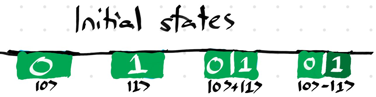
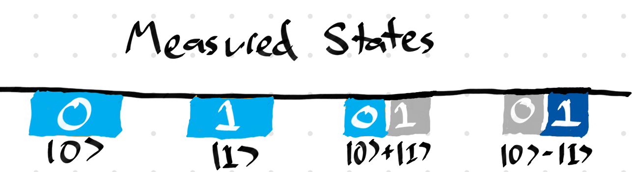
The basic state needed to show, at the very least, the probabilities of a bit being 0 or 1, and which bits are entangled with each other. To this end, I chose a simple representation that would show the relative probabilities of the state being |0> and |1>, without specifying all the pieces. I also chose to give negative pieces a slightly darker shade to differentiate them, which I use throughout the state representations.

Single bit states

The entangled connectors gain a slight curve here, so that complex entanglements are easily identified.

Simple entangled states

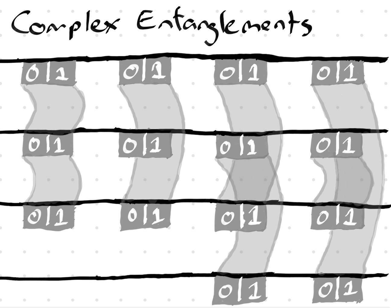Complex entangled states

Initial states are a nice green shade to differentiate them.

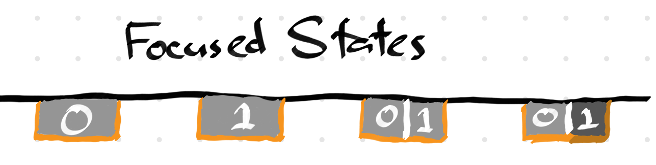
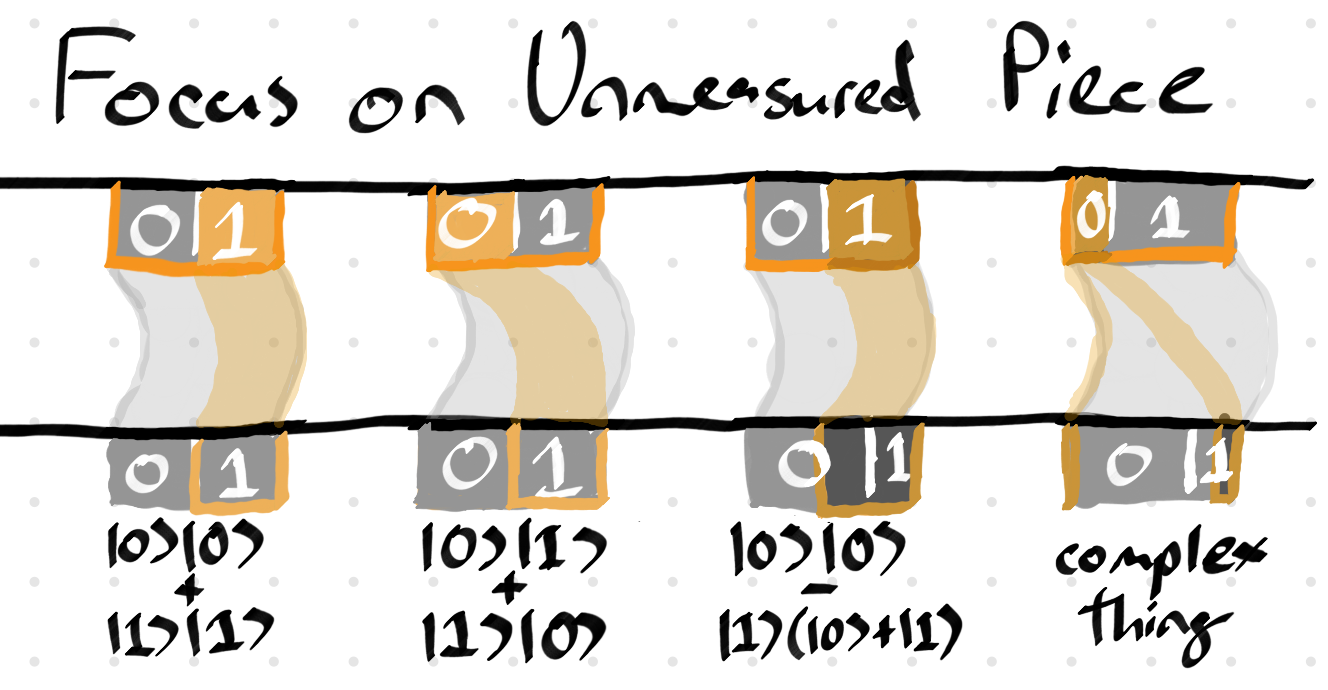
From there, a player can choose to focus on a state by clicking on it, which will highlight it and provide a textual explanation of the state.

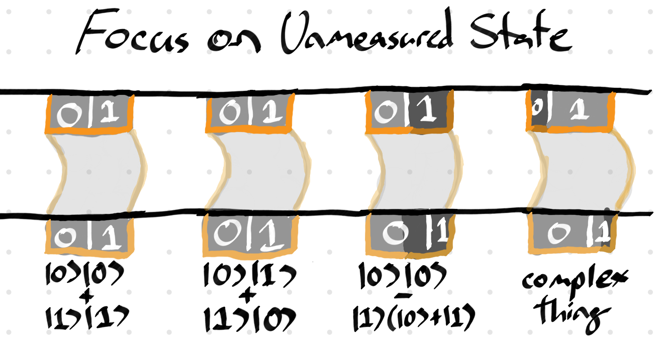
If the state is entangled, clicking again will focus on a piece of that state, showing how that piece relates to the states of entangled bits. Players can click on different pieces to examine them.

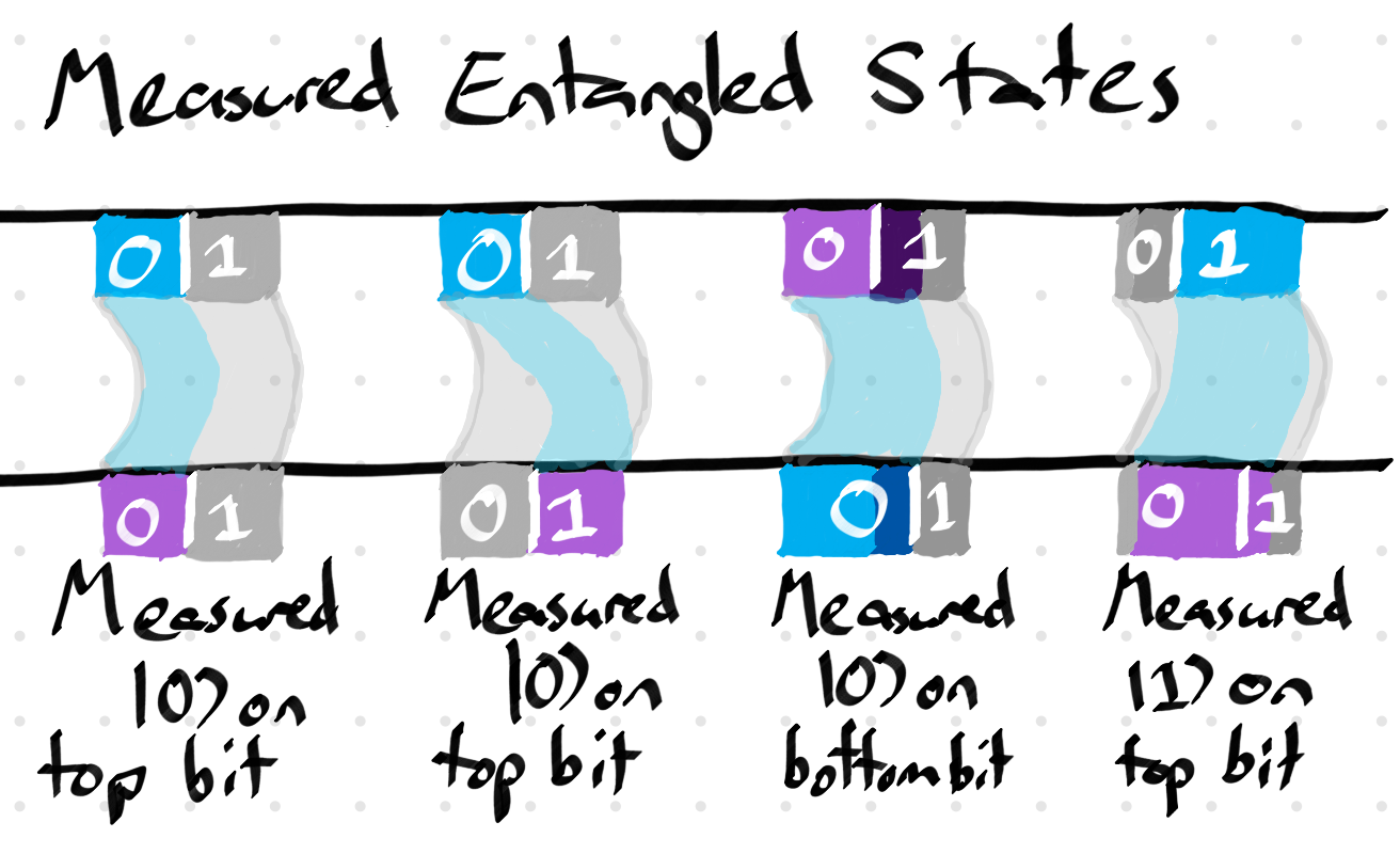
Measured states, as before, highlight the pieces which have been measured.

As before, measured entangled states highlight the pieces chosen on different bits in a slightly different colour. I’ve also connected the highlighted pieces so that entangled measured states stand out a bit more.

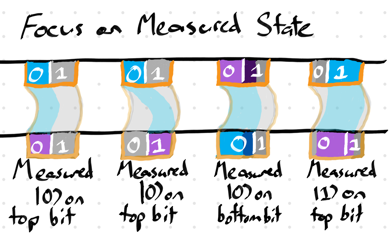
Finally, measured states can be focused on.

This leaves us with the following state diagram for our states (one of these things might need a new word).

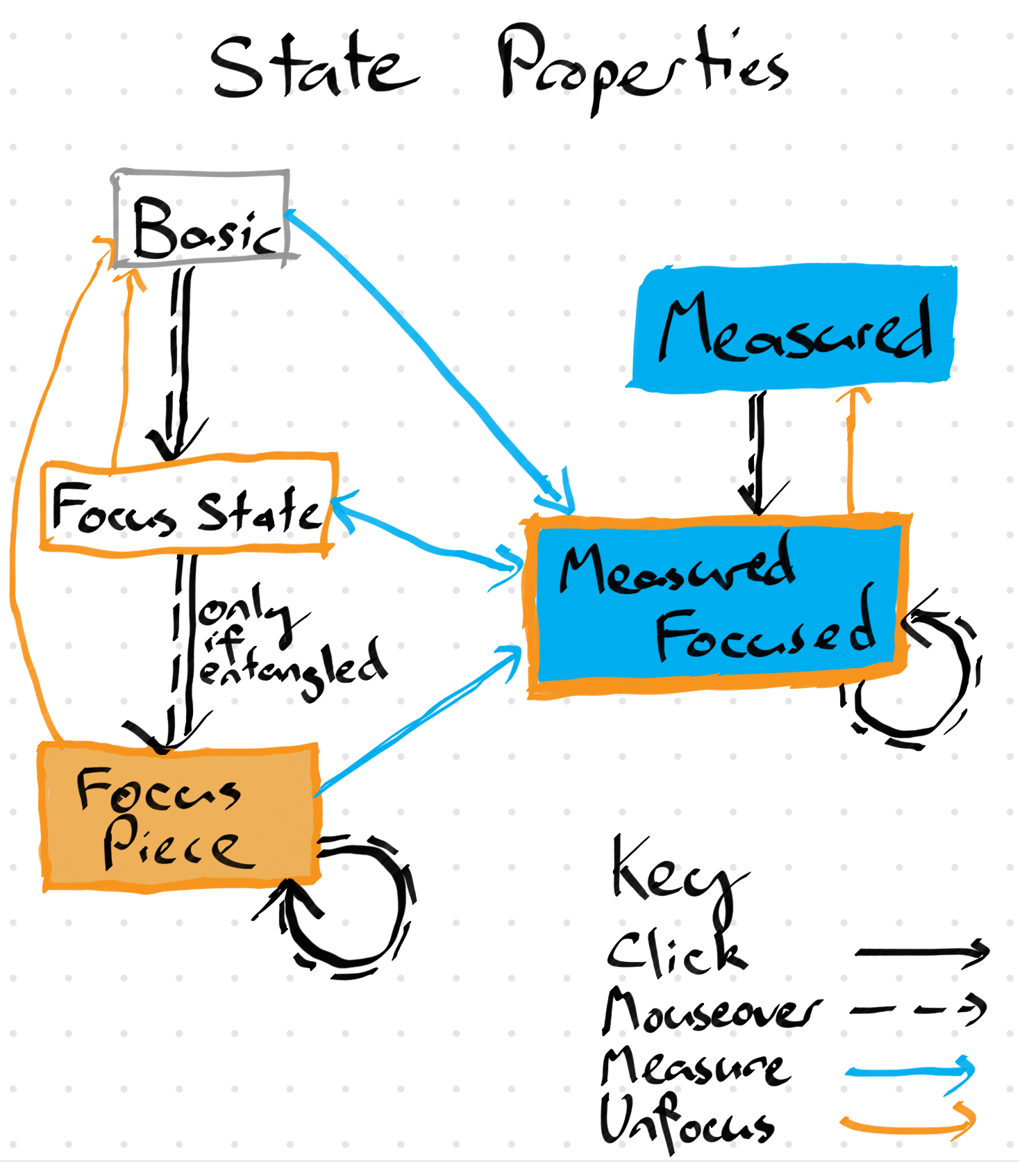A state representation state diagram. Mouse overs in this approach become ‘previews’ of a new state (in the case of measurements, it actually changes the measurement on mouseover but will then revert if you don’t click on it).

The pros of this representation are:

• States are a fixed size

• There’s less clutter on the screen

• The probabilities of |0> or |1> are front and centre, represented by a nice length model

• While the probabilities can still be small enough one of the “0” or “1” labels could be lost, only 1 of them can be like this

• Interrogating a state piece gives the player clear information about what measurements will do

• We lose a bit of information compared to the old visualisation, as we don’t see exactly which State Pieces relate to which other pieces (so, for instance, if a state has two |0> pieces, they get combined if that state is measured). I see this as a pro as this is extra, less important information.

• Negative state pieces are rendered subtly but consistently

And the cons:

• More reliant on colour than it should be (I’m probably going to have to do a pass that adds texture). And while I’m using Brewer Palettes for the colour choices (which makes my colours colour-blind friendly), I’m then adding shading to indicate all sorts of things which kind of ruins the whole point.

• There’s some inconsistency as to when pieces of the state can be focused on

• Having to click/tap twice to get piece information isn’t ideal

• I’ve been politely ignoring what happens when a player focuses on a state that is entangled with a measured state (ie. has purple bits). I’m currently thinking that I’ll overlay a focus over the measurement, but that gets a bit messy for my liking.

What I’ve done, and what’s next

Over the last couple of weeks, I’ve done a lot of refactoring of the quantum simulation model in order to allow this new view to work, and I’ve gotten started on the implementation. It’s been quite intense, but really worth it to have a cleaner, easier to use codebase. Right now, I’m working on code to allow players to choose which piece of a state gets measured, which has proven to be harder than expected.

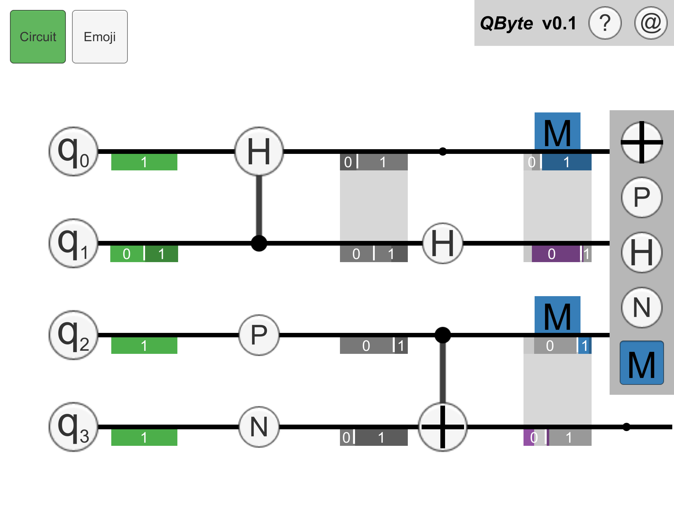The newest QByte build

I’ll probably be working on finishing up these state representations for the next week or two. After that, I’ll be working on some UI fixes, before coming back to the explanation engine.

That’s it for this week’s QByte devlog. Check out past posts and subscribe for updates here. If there’s anything you want to know about the project and how I’m making it, let me know in the comments or on twitter.